GPR 3D volume

The premise

This project has the main objective to create an open-source compatible processing pipeline to automatically elaborate Ground Penetrating Radar (GPR) data to output a GPR volume in VTK format. Once ready, the volume then can be used to intuitively localize, identify and analyze in 3D space buried objects in the top most layer of soil (in this case up to a depth of 1m).

GPR Data

GPR is a relatively new indirect non-invasive geophysical exploration method that can be used to acquire subsurface data up to a depth of 50m¹. This technique is based on the capture of reflected high frequency electromagnetic signals emitted from a controlled source. The contrast of electrical properties in the soil given by presence of anomalous objects, cavities, sedimentary structures, change in lithology or in water contents induce a variation in the signal’s propagation velocity thus producing a return pulse that is recorded. By visualizing the acquired data it is then possible to define the presence of perturbations across the medium and carry out different interpretations.

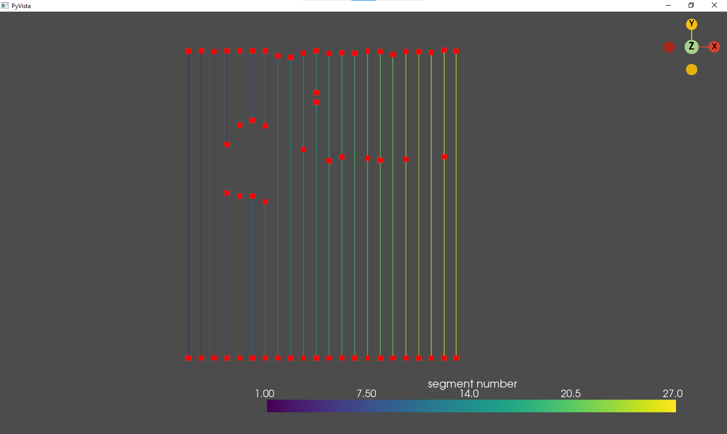
GPR data is recorded in traces grouped and organized in segments saved as SEGY files, every trace represents a point in space where the pulse has been emitted and the return signals recorded. A segment can be comprised of multiple sub-segments where the start and end (markers) can be defined during the recording or manually in the pre-processing phase. Markers can also be used to highlight points of interest encountered during the acquisition. These and any many other types of information are stored in the SEGY file header of both the segment and the single trace.

Processing pipeline

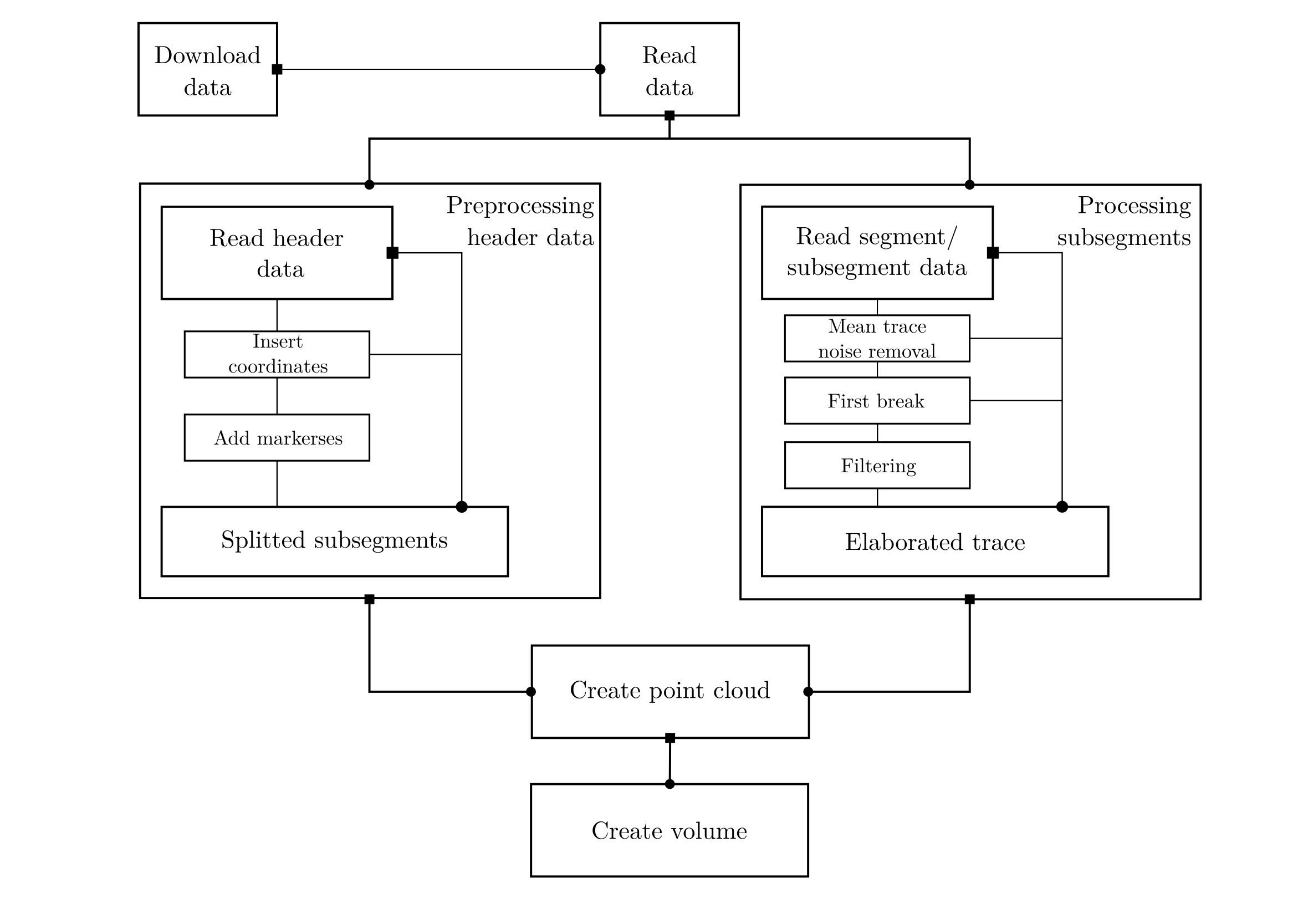
The processing pipline adopted to elaborate and visualize the data is composed by a pre-processing and processing phase. Once the data is downloaded the user needs to take in to account a series of characteristics. Firstly it is necessary to read the header to define the geometry of the survey using the trace position information and the presence of markers. If these types of information are present or not required, the pre-processing step can be skipped and the data directly used.

For every segment/sub-segment the returning signal data needs to be read and every trace has to be processed to a certain degree. It is better not to use the raw data or heavily processed data since the interpretation of both can result difficult. Signal noise can hide the objects or lead to wrong object geometry reconstruction and on the other hand too much processing/filtering can mask some objects or create artifacts also causing interpretation problems.

Once the header information is gathered and the signal data processed it is possible to create a uniform 3D point cloud. This is achieved by dividing the traces in multiple intervals (integration depth) and linearly interpolating on a 2D depth slice the mean trace intensities in the given depth interval². Although this approach effectively reduces the number of samples along the Z axis, thus lowering the vertical resolution of the model, it improves the overall quality of the data and highlights the presence of anomalies.

The intensity value of each point is then assigned to a cell (voxel) creating a GPR volume.

Results

This pipeline was applied to data acquired in Piazza della Scienza (Milan) to identify objects in the first meter of soil, important to the square’s future depaving and redesign project. The final computed GPR volume is 1m deep with a resolution of 600x600 cells giving a final grid resolution of 600x600x100. The grid, volume creation and final analysis were achieved using Pyvista. The code and data used to apply the different steps is available as a jupyter notebook. For a more in depth review of the process and more images a report in PDF format is available.